Track Cryptocurrency : Real-Time Insights with Dynamic Light and Dark Mode Dashboards in Power BI

How to Import Cryptocurrency Data Using Python: A Step-by-Step Guide

Are you looking to integrate cryptocurrency data into your analysis?

This blog post explores using Python scripts to automate the import process, making it easier to track and analyse crypto market trends.

Step 1: Convert ‘YYYY-MM-DD’ to UNIX Timestamp

Yahoo Finance uses UNIX timestamps to specify date ranges for historical data. We'll start by converting a date in the format `YYYY-MM-DD` to a UNIX timestamp.

import time

def date_to_unix(date_str):
    return 
int(time.mktime(time.strptime(date_str, "%Y-%m-%d")))

# Example

start_date = '2023-07-01'

unix_start_date = date_to_unix(start_date)

print(f"Start Date: {start_date} -> UNIX Timestamp: {unix_start_date}")

Output:

Start Date: 2023-07-01 -> UNIX Timestamp: 1688169600

Step 2: Get the Current Date in ‘YYYY-MM-DD’ Format

Next, we fetch the current date to use it as the end date for fetching historical crypto data.

from datetime import datetime

current_date = datetime.now().strftime('%Y-%m-%d')

unix_current_date = date_to_unix(current_date)

print(f"Current Date: {current_date} -> UNIX Timestamp: {unix_current_date}")

Output:

Current Date: 2024-07-28 -> UNIX Timestamp: 1722124800

Step 3: Read the CSV File to Get the List of Crypto Symbols

We store the crypto symbols (trackers) in a CSV file, which we'll read into a data frame.

import pandas as pd

file_path = 'path/to/your/csvfile.csv'

symbols_df = pd.read_csv(file_path)

trackers = symbols_df['Symbol'].tolist()

print("Crypto Symbols:")

print(trackers)

Output:

Crypto Symbols:
['BTC-USD', 'ETH-USD', 'XRP-USD', 'LTC-USD']

Step 4: Initialize a List to Hold All Data

We'll create an empty list to store the DataFrames for each crypto's historical data.

data_frames = []

Step 5: Fetch Data from Yahoo Finance

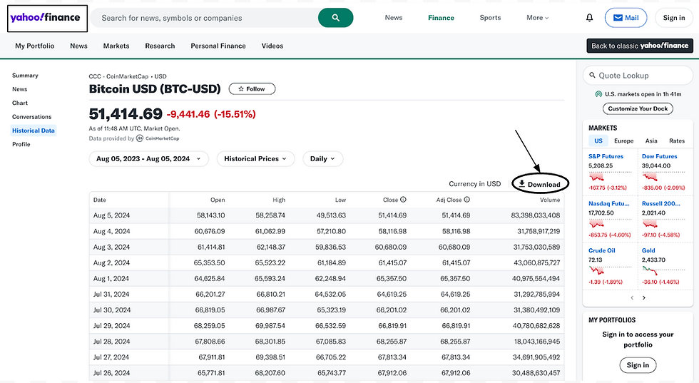
Now, we'll loop through each crypto symbol, construct the URL for Yahoo Finance, fetch the historical data, and store it in a data frame.

period1 = date_to_unix(start_date)
period2 = date_to_unix(current_date)

for tracker in trackers:

    url = f'https://query1.finance.yahoo.com/v7/finance/download/{tracker}?period1={period1}&period2={period2}&interval=1d&events=history&includeAdjustedClose=true'

    try:

        df = pd.read_csv(url)

        df['Symbol'] = tracker

        data_frames.append(df)

        print(f"Data for {tracker} downloaded successfully.")

    except Exception as e:

        print(f"Failed to download data for {tracker}: {e}")

Output:

Data for BTC-USD downloaded successfully.

Data for ETH-USD downloaded successfully.

Data for XRP-USD downloaded successfully.

Data for LTC-USD downloaded successfully.

Step 6: Concatenate All DataFrames into a Single DataFrame

Once all data has been fetched and stored in individual DataFrames, we concatenate them into a single DataFrame.

combined_data = pd.concat(data_frames, ignore_index=True)
combined_data = combined_data[['Symbol', 'Date', 'Open', 'High', 'Low', 'Close', 'Adj Close', 'Volume']]
print(combined_data.head())

Output:

   Symbol        Date       Open       High        Low      Close  Adj Close     Volume

0  BTC-USD  2023-07-01  192.020004  194.610001  191.889999  192.460007  191.362930  59021500

1  BTC-USD  2023-07-02  190.850006  193.160004  190.179993  192.800003  191.700000  48655000

2  BTC-USD  2023-07-03  192.470001  193.490005  192.100006  193.240005  192.150009  37538000

3  BTC-USD  2023-07-04  193.169998  194.479996  192.479996  193.149994  192.060000  50777000

4  BTC-USD  2023-07-05  192.800003  195.029999  192.600006  194.169998  193.070000  55548000

Full Script after merging above code:

import pandas as pd

import time

from datetime import datetime

def date_to_unix(date_str):

    return int(time.mktime(time.strptime(date_str, "%Y-%m-%d")))

current_date = datetime.now().strftime('%Y-%m-%d')

start_date = '2023-07-01'

period1 = date_to_unix(start_date)

period2 = date_to_unix(current_date)

file_path = 'path/to/your/csvfile.csv'

symbols_df = pd.read_csv(file_path)

trackers = symbols_df['Symbol'].tolist()

data_frames = []

for tracker in trackers:

    url = f'https://query1.finance.yahoo.com/v7/finance/download/{tracker}?period1={period1}&period2={period2}&interval=1d&events=history&includeAdjustedClose=true'

    try:

        df = pd.read_csv(url)

        df['Symbol'] = tracker

        data_frames.append(df)

        print(f"Data for {tracker} downloaded successfully.")

    except Exception as e:

        print(f"Failed to download data for {tracker}: {e}")

combined_data = pd.concat(data_frames, ignore_index=True)

combined_data = combined_data[['Symbol', 'Date', 'Open', 'High', 'Low', 'Close', 'Adj Close', 'Volume']]

print(combined_data.head())

Why Use a Date Time Period Slicer?

A date-time period slicer offers several benefits:

Dynamic Time Periods: Allows users to analyze data across various time frames without manually selecting date ranges.

Improved Insights: Facilitates quick comparison of different periods, enabling better decision-making.

Ease of Use: Simplifies data interaction for end-users, enhancing the overall experience in Power BI dashboards.

Custom Reporting: Tailors reports to specific business needs, such as comparing recent performance to historical trends.

Setting Up Your Power BI Environment

Before we begin, ensure that you have the following:

Power BI Desktop: Download and install it from the official Power BI website.

Sample Dataset: Use a stock data sample that includes a Date column to apply the slicer.

Creating the Date Category DAX Formula

To create an advanced date time period slicer, write a DAX formula that categorizes each date into a specific time period. Here’s the process:

Step 1: Open Power BI Desktop

Launch Power BI Desktop and load your dataset. Ensure your dataset contains a Date column for the slicer.

Step 2: Create a New Column in Your Data Model

Go to the “Data” view.
Select the table containing your date column (e.g., Stocks Data).
Click on “New Column” in the ribbon.
Enter the following DAX formula:

DAX

Date Category = 

VAR TodayDate = TODAY()

VAR StartOfYears = DATE(YEAR(TodayDate), 1, 1)

VAR FiveDaysAgo = TodayDate - 7

VAR ThreeMonthsAgo = EOMONTH(TodayDate, -3) + 1

VAR SixMonthsAgo = EOMONTH(TodayDate, -6) + 1

VAR OneYearAgo = EOMONTH(TodayDate, -12) + 1

VAR FiveYearsAgo = EOMONTH(TodayDate, -60) + 1

VAR MaxDate = CALCULATE(MAX('Stocks Data'[Date]), ALL('Stocks Data'[Date]))

RETURN

    SWITCH(

        TRUE(),

        'Stocks Data'[Date] > TodayDate, "Future",

        'Stocks Data'[Date] >= TodayDate, "Today",

        'Stocks Data'[Date] >= FiveDaysAgo && 'Stocks Data'[Date] < TodayDate, "5D",

        'Stocks Data'[Date] >= ThreeMonthsAgo && 'Stocks Data'[Date] < TodayDate, "3M",

        'Stocks Data'[Date] >= SixMonthsAgo && 'Stocks Data'[Date] < ThreeMonthsAgo, "6M",

        'Stocks Data'[Date] >= StartOfYears && 'Stocks Data'[Date] < TodayDate, "YTD",

        'Stocks Data'[Date] >= OneYearAgo && 'Stocks Data'[Date] < StartOfYears, "1Y",

        'Stocks Data'[Date] >= FiveYearsAgo && 'Stocks Data'[Date] < OneYearAgo, "5Y",

        'Stocks Data'[Date] >= MaxDate && 'Stocks Data'[Date] < FiveYearsAgo, "Max",

        "Older"

    )

Explanation of the DAX Formula

The provided DAX formula categorizes dates into various time periods. Let's break down each part of the formula:

Variable Definitions

1. TodayDate:

VAR TodayDate = TODAY()

Retrieves the current date using the `TODAY()` function.

2. StartOfYears:

VAR StartOfYears = DATE(YEAR(TodayDate), 1, 1)

Calculates the start of the current year by setting the month and day to January 1st of the current year.

3. FiveDaysAgo:

VAR FiveDaysAgo = TodayDate - 7

Computes the date five days prior to today.

4. ThreeMonthsAgo:

VAR ThreeMonthsAgo = EOMONTH(TodayDate, -3) + 1

Determines the date three months ago, set to the first day of the month.

5. SixMonthsAgo:

VAR SixMonthsAgo = EOMONTH(TodayDate, -6) + 1

Identifies the date six months ago, set to the first day of the month.

6. OneYearAgo:

VAR OneYearAgo = EOMONTH(TodayDate, -12) + 1

Finds the date one year ago, set to the first day of the month.

7. FiveYearsAgo:

VAR FiveYearsAgo = EOMONTH(TodayDate, -60) + 1

Establishes the date five years ago, set to the first day of the month.

8. MaxDate:

VAR MaxDate = CALCULATE(MAX('Stocks Data'[Date]), ALL('Stocks Data'[Date]))

Retrieves the maximum date in the dataset to categorize any dates older than five years.

Visualizing Cryptocurrency Data in Power BI

One of the standout features of our Power BI dashboard is the dynamic visualization using light and dark modes, achieved through innovative use of layers and shapes. Here are the key points:

Dynamic Visual Modes:

Utilizes both light and dark modes for enhanced user experience.

Achieved through innovative use of layers and shapes.

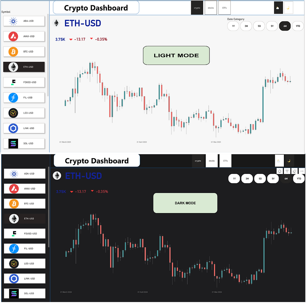
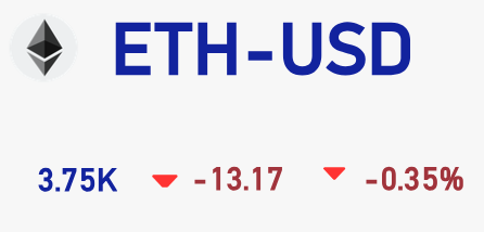
Real-Time Data Updates:

Displays daily profit and loss for selected cryptocurrencies.
Requires an active internet connection for live data updates.

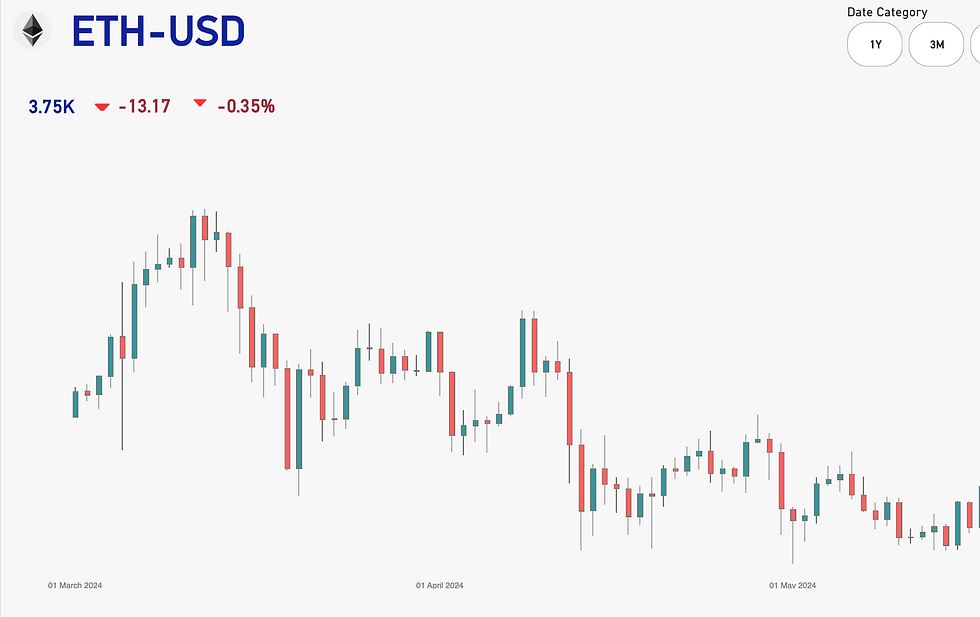
Advanced Date Category Slicer:

Offers various time frames: 3 days, 5 days, 3 months, 6 months, and 1 year.
Allows users to analyze trends and patterns over different periods.

Candlestick Chart Visualization:

Used to display the value fluctuations of the selected cryptocurrency.
Showcases open, high, low, and close values for comprehensive market behaviuor insights.

Interactive Slicer:

Users can select a cryptocurrency from the slicer to view live data updates.
Provides up-to-the-minute information for informed decision-making.

Comprehensive Tabs:

Includes three tabs for a broader range of data: Stocks, ETFs, and Cryptocurrencies.
Ensures a holistic approach to market analysis.

This combination of real-time data, dynamic visual modes, and comprehensive time period analysis makes the Power BI dashboard a powerful tool for monitoring and understanding the ever-changing cryptocurrency market.

Link of Dashboard - link

Resources from The Developer

Track Cryptocurrency : Real-Time Insights with Dynamic Light and Dark Mode Dashboards in Power BI

Recent Posts

Comments

CONTACT US